Helmholtz Equation: Steady-Periodic

K. D. Cole

In this section, steady-periodic heat conduction is treated. Also called time-harmonic or thermal-wave behavior, this special case is important whenever the causal effect is harmonic in time and has continued long enough for any start-up transients to die out.

Rectangular Coordinates. Steady-periodic 1-D.

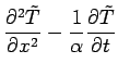
Consider a one-dimensional region in which the temperature is sought. The transient temperature distribution satisfies

$$\frac{\partial^2 \tilde{T}}{\partial x^2} - \frac{1}{\alpha} \frac{\partial \tilde{T}}{\partial t} = \frac{1}{k}\tilde{g}(x,t)$$ (1)

$$k_i \frac{\partial \tilde{T}}{\partial n_i} + h_i \tilde{T} = \tilde{f}_i(t); \;\; \mbox{at boundary }\;i=1,2$$

Here $\alpha$ is the thermal diffusivity (m$^2 \cdot$ s$^{-1}$), $k$ is the thermal conductivity (W$\cdot$m$^{-1}\cdot$K$^{-1}$), $\tilde{g}$ is the volume heating (W$\cdot$ m$^{-3}$), and $\tilde{f}_i$ is a specified boundary condition. Index $i = 1,2$ represents the boundaries at the limiting values of coordinate $x$. The boundary condition may be one of three types at each boundary: boundary type 1 is specified temperature ($k_i=0$ and $h_i=1$); boundary type 2 is specified heat flux ($h_i=0$); and, boundary type 3 is specified convection where $h_i$ is a constant-with-time heat transfer coefficient (or contact conductance).

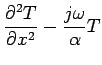
Since in this section the applications of interest involve steady-periodic heating, the solution is sought in Fourier-transform space, and the solution is interpreted as the steady-periodic response at a single frequency $\omega$. For further discussion of this point see Mandelis (2001, page 2-3). Consider the Fourier transform of the above temperature equations:

$$\frac{\partial^2 T}{\partial x^2} -\frac{j \omega}{\alpha}T = - \frac{1}{k} g(x,\omega )$$ (2)

$$k_i \frac{\partial T}{\partial n_i} + h_i T = f_i(\omega); \;\; \mbox{at boundaries } \;\; i=1,2$$

Here $T$ is the steady-periodic temperature, $g$ is the steady-periodic volume heating, $f_i$ is the steady-periodic specified boundary condition, and $j = \sqrt{-1}$.

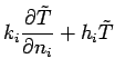
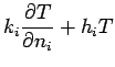
The temperature will be found with the Fourier-space Green's function, defined by the following equations:

$$\frac{\partial^2 G}{\partial x^2} -\sigma ^2 G = - \frac{1}{\alpha} \delta(x-x')$$ (3)

$$k_i \frac{\partial G}{\partial n_i} + h_i G = 0; \;\; i=1,2$$ (4)

Here $\sigma^2 = j \omega/ \alpha$ and $\delta(x-x')$ is the Dirac delta function. The coefficient $1/ \alpha$ preceding the delta function in Eq. (3) provides the 1-D frequency-domain Green's function with units of s$\cdot$m$^{-1}$. This is consistent with earlier work with time-domain Green's functions.

If the steady-periodic Green's function $G$ is known (given below), then the steady-periodic temperature is given by the following integral equation:

$$T(x,\omega) = \frac{\alpha}{k} \int g(x',\omega) G(x,x',\omega) d x' \;\; \mbox{ (for volume heating)}$$

$$+ \alpha f_i(\omega) \times \left[ \begin{array}{ll} \partial G /... ...}{k} G(x, x_i, \omega) & \mbox{(type 2 or 3)} \end{array}\right] \;\;\; i = 1,2$$ (5)

For a derivation of this equation see Beck et al. (1992, pp. 40-43). Next the steady-periodic Green's functions are given for 1-D bodies for cases XIJ.